Monday, May 16, 2016

Raster Modeling


Goals: 
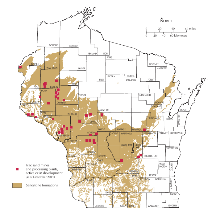
The goal of this lab was to use multiple geoprocessing tools to build models for sand mining suitability as well as sand mining impacts on the environment and culture in Trempealeau County, Wisconsin.

In this exercise, I had to build a sand mining suitability model, build a sand mining risk model, and overlay the two models to find the best locations for sand mining with minimal environmental and community impacts.


Data Sets and Sources:
The data sets and sources used for this lab were from Trempealeau county public database, NLCD land use data, USGS DEM data, and water table data from the Wisconsin Geological and Natural History Survey.


Objectives:
Suitability Model

Objective 1: The first objective was to find suitable land based on geological criterion. I converted a Trempealeau County geology feature class to a raster. I then performed a reclass which ranked the geologic formations based on their suitability. The process is shown in the below model.
Objective 2: The second objective was to find suitable land based on the land use criteria. I ranked each land use type based on what I thought was most suitable using the reclassify tool. My rankings are listed below.
3: Barren Land, Herbaceuous, Hay, Pasture, Cultivated Crops
2: Shrub, Scrub 2
1: Deciduous Forest, Evergreen Forest, Mixed Forest
For Open Water, Developed, Open Space Developed, Low Intensity Developed, Medium Intensity Developed, High Intensity, Woody Wetlands I assigned 0 to exclude these from my suitability results. 

Objective 3: The third objective was to find suitable land based on the proximity to railroad terminals. I performed a Euclidean distance tool, and assigned values of 1, 2, and 3 using the reclassify tool.
Objective 4: The fourth objective was to find suitable land based on slope. I ran the slope calculator tool on the Trempealeau county DEM file which gave me a percent rise.
Objective 5: The fifth objective was to rank areas of land where the water table is closer to the surface. In order to do this, I needed coverage files from the WI Geological Survey website. I then had to import them into my geodatabase before creating a raster from the contour lines using the topo to raster tool. I once again ranked and reclassed the results.
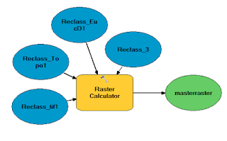
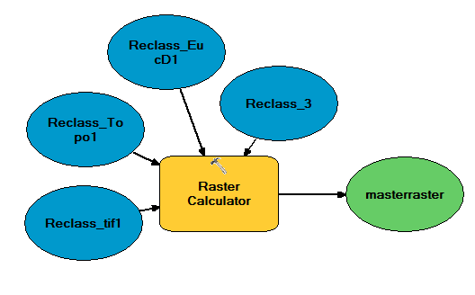
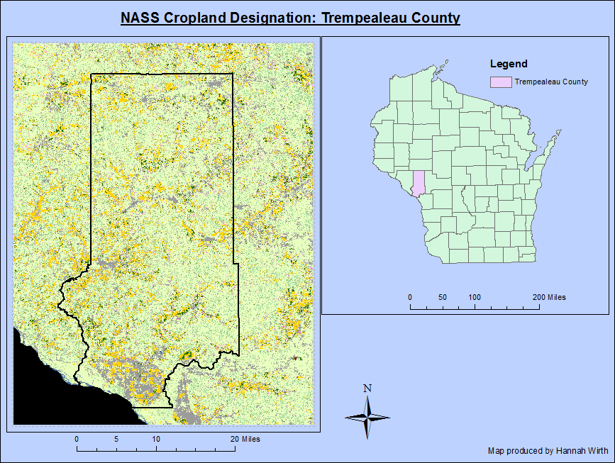
Objective 6: The sixth objective was to combine all of the objectives into one index model that adds up all of the ranks I had assigned in each of them. I used raster calculator to create a master raster of the criteria. The suitability map is figure 1 shown below.
Figure 1: This map is a suitability model for sand mining in Trempealeau County
Objective 7: The task for objective seven was to exclude all land uses that were not suitable to include in the suitability model. These included: open water, developed land, and woody wetlands. I already excluded the unwanted data in objective two.


Impact Model

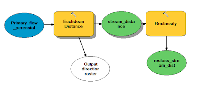
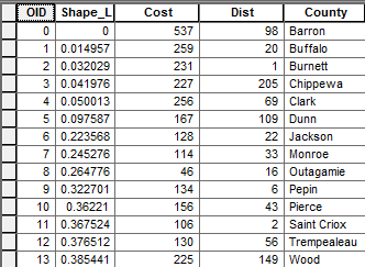
Objective 8: The eighth objective included using a DNR-hydro feature class to see the environmental impact potential in the areas where sand mining operations occur. I only included primary flow perennial streams. I then used the euclidean distance tool to calculate and reclassify the distances in the same three criteria as before (3=High, 2=Medium, and 1=Low).
Objective 9: In the ninth objective, I projected a prime farmland feature class before converting it to a raster. Next, I used the reclass tool to rank the land based on land that was prime farmland (or valuable farmland).
Objective 10: In objective ten, I had to determine the impact based on distance to residential or populated areas. I used a feature class containing corporate district limits. Next, I performed euclidean distance on it, making sure that no sand mines are within 640 meters of a residential area. The three distance classifications represent a dust shed for potential mines.

Objective 11: Objective eleven was to determine potential impact on schools. This meant starting with the parcels feature class and querying all parcels that contained the word 'school'. Then, I created a new feature class with property owned by schools. After that I used the euclidean distance tool and reclassified the results into the three rankings.
Objective 12: For objective twelve, I chose to look at parks in Trempealeau County. I used the euclidean distance tool and reclassify tool on the parks feature class to determine impact rankings.

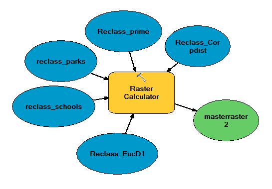
Objective 13: Objective thirteen was to calculate risk. The idea is the same as the first suitability model. I am used raster calculator to add up the values in each raster to determine the impact.
Overlay

Objective 14: The final objective was to overlay the two models together. The final outcome shows where to find best locations for sand mining with minimal environmental and community impact. In order to do this, I had to subtract the environmental impact raster from the suitability raster. This map is in the results section.

Objective 15: The Python script for this exercise is the third script in the "Python Script" post in this blog.


Results: The final map (figure 2 down below), was an overlay between the suitability model and the environmental impact model. Everything in green signifies an area of high suitability and low environmental impact. Areas that are red signify low suitability with high environmental impact.
Figure 2: This is the map of the suitability model and the environmental impact model combined
It is interesting to see the final model and what it represents. This is a map produced with real data, but is no means an answer to suitability/environmental impact problems. The area of green and a little bit of the orange are areas of high suitability. Areas in red are areas that have low suitability and high environmental impacts.

Conclusion: The final suitability and environmental impact model is a collective map of 10 rasters calculated through ArcMap. While working with raster modeling, I have learned how to properly take a feature class and convert it into a raster. I have also learned how to  run the Euclidean Distance tool to create a raster of an area. The other major tool I learned to efficiently use was the reclassify tool. This tool makes it possible to use the raster calculator mathematics on rasters that are uniform. The geoprocessing tools use simple mathematics equations to create raster data that is extremely useful. 


Friday, April 22, 2016

Network Analysis


Goals and Objectives: The goal of this assignment is to learn how to perform network analysis. In the first part of this assignment, we had to write a python script to select the mines that would be used for network analysis. We are trying to figure out what the hypothetical cost is on the roads the trucks use to transport sand from the mine to the rail station.

Methods: The beginning of this project was getting a python script ready to use for network modeling. Once that was complete, we used network modeling to do efficient route modeling. The main tool we used was "find nearest facility". We used this is find the nearest rail station to the sand mines. The network dataset that contains the roads came from ESRI streetmap, the mine data came from the Wisconsin DNR, and the rail data came from the Department of Transportation.

Next, was to create a data flow model. By creating the data flow model, I could clearly see what the exact steps were in the modeling process.
Figure 1: The data flow model above shows the step-by-step actions I took to get my results

Figure 2: The map above shows the routes the trucks have to use to get the sand to the rail stations.
Source: ESRI street map USA
The map above shows where the rail stations are as well as where the mines are. The map also shows the truck routes taken from the mine sites to the rail stations and back again. The constant driving with heavy material back and fourth causes stress on the roads. The table below shows how each county in Wisconsin is affected by the trucks driving on public roads. 

Figure 3: The table above is the final product showing the county, cost of road repair, and the distance the truck has to travel.
Conclusion:
After analyzing the results, I can't help but wonder how the counties plan on paying for the roads. It does not make sense for the taxpayers to pay the bill when the trucks from the mining companies are the vehicles doing the most damage on the roads. 
Once the background is set for network analysis, it is a very useful tool to help map out a potential route for something. This project was interesting and important because it is such a large scale local problem. 

Sources:
ESRI street map USA
Wisconsin DNR
Department of Transportation


Friday, April 8, 2016

Data Normalization, Geocoding, and Error Assessment for Western Wisconsin Sand Mine Locations


Goals and Objectives:

The main goal for this assignment is to geocode the locations of all the sand mines in Western Wisconsin and compare the results. The six main objectives for this exercise are the following: normalize the mine locations in the MS Excel table, connect to the geocoding service from ESRI and geocode the 16 mines that were given to you, connect to the ArcGIS online server for UWEC and add the PLSS feature class, manually locate the mines from your 16 that have a PLSS location, and finally compare your results with the results of the other students in class. In order to reach the end goal, it was critical to know how to normalize the data that was given to us. Once the data was normalized, it made geocoding much easier and more accurate.


Methods:

The first step in the geocoding process was to normalize the data. Figure 1 shows how the data was given to us from the Wisconsin DNR. The address information was not uniform. Some had the PLSS address, some had the actual address, and some had both. Figure 2 shows the data after it has been normalized. The data in figure 2 is ready to be geocoded. Once the normalized data is imported into ArcMap, the geocoding process can begin.

Figure 1. The data was given to us in an Excel table and was not normalized

Figure 2. The data has been normalized and is ready for geocoding
Once all of the points were geocoded, it was time to gather everyone's data from a shared location. I merged the data and queried out the mine locations that were in common with my mine locations.


Results:

After trial and error with different tools, I was able to figure out my mine locations in comparison to my classmates' mine locations. The point distance tool was useful to see the amount of error that occurs from person to person. Error is inevitable in geocoding locations.
Figure 3. This is a map of my geocoded mines as well as five of my classmates geocoded mines
Source: Wisconsin DNR

Discussion/Conclusion:

There were two different ways of geocoding the mine locations. The easiest way was using the address provided by the Wisconsin DNR. The other way was taking the PLSS address and figuring out where it is on the map. Some of the places were difficult to find on the background map, so I had to use Google Earth to find out where the mine is and then match it in ArcMap.

In figure 3 it is apparent that not all of the locations were geocoded exactly the same. There is distance error for every mine site.

The most frustrating thing about this project was getting all of the shapefiles merged into one shapefile. The data was not normalized because we all took different approaches in geocoding our mine locations. It is important to understand how difficult it can be to normalize and merge data. The feeling of success after struggling is great. This was a very stressful yet rewarding assignment.

Sources:

Google Maps- https://www.google.com/maps

ESRI Online- http://www.esri.com/software/arcgis/arcgisonline 

Wisconsin DNR- http://dnr.wi.gov/ 


Wednesday, March 16, 2016

Mapping the Downloaded Data for the Sand Mining Suitability Project

Exercise 5: Mapping the Downloaded Data for the Sand Mining Suitability Project

Goals and Objectives: The goal of exercise 5 was to become more familiar with downloading data from different sources on the internet, importing the data to ArcGIS, joining data, projecting data from these different sources into one coordinate system. The final task was to build and design a geodatabase to store the data.

General Methods: The first part of this exercise consisted of downloading data about Trempealeau county from the internet. Before any downloading began, a temporary file had to be set up in the temp folder because some of the data takes up a lot of computer space. From the temp folder, I extracted the data into a working folder. All of the data for this exercise were gathered off of the internet. The sources and the data taken from that website are listed below.

Sources and Data Downloaded:

  • US Department of Transportation-- Railroads
  • USGS-- Digital Elevation Model
  • USDA-- Land Use and Land Cover
  • USDA NRCS Soil Survey-- Soil Information
  • Trempealeau County Land Records-- Trempealeau County Geodatabase
After all of the data was downloaded and in the correct folders and the geodatabase was organized, the Python Script was written. A screen shot of that script can be seen in my blog titled "Python Script". From the Python Script in post two the following maps were created:
Figure 1: Cropland Data for Trempealeau County

Figure 2: Land Cover Data for Trempealeau County

Figure 3: Digital Elevation Model (DEM) for Trempealeau County


Data Accuracy:

By looking at the metadata for the data downloaded, it shows information about the actual data gathered. It also shows how accurate and reliable the data is. This is helpful to know about any limitations or coordinate system projections for the future. Below is a list of the data gathered. For each data set, we had to find the scale, effective resolution, minimum mapping unit, planimetric coordinate accuracy, lineage, temporal accuracy and attribute accuracy. If there was no information for a category, it is denoted with N/A.


Conclusion: The ability to download free data off of the website from credible sources is a great skill to have. Most of the data that will be needed to complete this project has now been downloaded. It is all stored in a geodatabase specifically for this project. Although the downloading of data can be frustrating, it is good practice. I am very interest and curious to see what the final results show about the suitability of frack sand mining in Trempealeau County.


Websites:
USDOT:  http://www.rita.dot.gov/bts/sites/rita.dot.gov.bts/files/publications/national_transportation_atlas_database/index.html
USGShttp://nationalmap.gov/about.html
USDAhttp://datagateway.nrcs.usda.gov/
USDA NRCS Soil Surveryhttp://websoilsurvey.sc.egov.usda.gov/App/HomePage.htm
Trempealeau County Geodatabasehttp://www.tremplocounty.com/tchome/landrecords/


Tuesday, March 15, 2016

Python Script

Python Script #1

The goal for exercise 5 part three was to write a new Python script to project, clip, and load all the data into a geodatabase. 

Python is a general-purposed programming language. It is designed to have readable code and syntax that programmers can use. In our GIS II class, we used Python to  write scripts for our geodatabases in ArcGIS. For this specific assignment, we had to download multiple data and rasters to analyze Trempealeau county. We used Python for projecting the rasters into the Trempealeau geodatabase. 

Figure 1: This is a screenshot of the completed Python script 
Above is the completed Python script. The Python troubleshooting took quite a long time and tested my patience. When there were no longer any errors with the script, it was complete.

Python Script #2

The goal of exercise 7 was to write a python script to prepare the data for network analysis. Python Scripter was used to write the script. The script consisted of selecting the mines, multiple queries, and selecting by location. I used select by location to find the mines that were active, within 1.5 km of a rail system, and a mine that does not have a rail loading station on-site.

Figure 2: This is the completed Python script for exercise 7

Writing the script was frustrating, but once I got the hang of it, it was easier to write. The script was broken down into    main parts. Step one was to set up the environments and prepare for writing the SQL statements. Step two was to write three SQL statements. Step three was to create new feature from the SQL expressions. Step four was to select by location to find the number of mines that are active, within 1.5 km of a rail system, and find mines that do not have a rail loading station on-site. I found 35 mine systems that require trucking to and from their sites. 

Python Script #3

This is the last and final Python script for GIS II. I went through the same workflow as I did in ArcMap. This script created a new raster overlay based on the same criteria, but one weighted 1.5 times more than the others. I chose to weight distance from streams higher. The Python script is shown below.

Figure 3: This is the completed Python script for exercise 8


Thursday, February 25, 2016

Sand Mining in Western Wisconsin--Overview


Sand Mining in Western Wisconsin

Background Information:
        Recently, sand mining in Wisconsin has had a dramatic increase in popularity. The sand mined in Wisconsin is ideal for hydraulic fracturing. Hydraulic fracturing, also known as fracking, is the process of cracking or fracturing the rock formations beneath the surface of the earth to extract natural gas or crude oil. Water is blasted at high speeds to crack the rock. This is where the sand comes into play. Once the fissures, or small cracks in the rock have been formed, sand is sent into the cracks made in the rock and is used as a wedge to keep the crack open. The smaller the sand particles the better because they can get wedged into smaller cracks compared to the large particles. The image below (figure 1) shows how the drilling and fracturing works. The small white dots in the image represent the sand that holds open the newly formed cracks.
Figure 1: An animated picture of the hydraulic fracturing process
What is frac sand mining?
        Frac sand mining is the mining of sand the fracturing companies use to hold open the fissures they make in the rock. Frac sand is actually very small pieces of quartz, also known as silicon dioxide (SiO2) which is more commonly known as silica sand. The individual particles of sand are spherical and extremely durable as seen in the picture below.

Figure 2: An up close image of silica sand. As you can see,
the individual granules of sand are very spherical.
Since the sand needed for fracking is very specific, it is only found in a few places. In the United States, the Midwest (specifically Wisconsin and Minnesota) contain vast deposits of the sand. In order to reach the sand, the mining companies must clear the overburden (topsoil, clay, silt, and/or loam). The actual extracting of the sand is then done with a possibility of blasting depending on how hard the silica is. After the sand is extracted, the sand is then washed with water and chemicals, dried in large rotating drums, and finally screened and sorted for selling.

Where is frac sand mining in Wisconsin?
       The image below is a map of where frac sand mines are in Wisconsin. The red squares are frac sand mines as of December 2011. The area shaded in beige is the area where there is sandstone to possibly be mined. Wisconsin has some of the best frac sand because of geologic formations that are close to the surface. Wisconsin hold 75% of the frac sand mining market in the United States.
Figure 3: A map of the frac sand sites in Wisconsin

Issues associated with frac sand mining:
      There are many issues with frac sand mining, the biggest being public health and air/water quality. Since hydraulic fracturing and frac sand mining is a new industry, it is very poorly regulated. There are very few rules and regulations that hold the companies accountable.
      With Wisconsin's open-pic sand mines, it exposes surrounding citizens to toxic chemicals and airborne matter that is damaging to lungs. Inhaling silica can cause silicosis which is an incurable disease and can cause cancer. The mine workers are exposure is regulated by the government because of this danger, but there is no limits or regulations for the general public.
      Another issue with frac sand mining is the damage the trucks and machinery do to the surrounding infrastructure. With large trucks, semis, and machines driving to-and-from the sand sites, the local roads, which were not built to hold extreme amounts of weight, are deteriorating at a rapid rate.

How can GIS be used to further explore issues with frac sand mining?
     Geographic Information Systems, GIS, can be used to help elevate some of the current problems with frac sand mining. Along with mapping where the actual mining sites are, GIS can be used to show potential problem areas. One issue GIS could help solve is the problem with infrastructure. With GIS one could map out the best and most practical route to take to and from sand mining sites to railways. A GIS could also map out a potential buffer around sand mining sites to showing the public the health risks associated with being close to a site.

Sources: