Mapping the Downloaded Data for the Sand Mining Suitability Project

Exercise 5: Mapping the Downloaded Data for the Sand Mining Suitability Project

Goals and Objectives: The goal of exercise 5 was to become more familiar with downloading data from different sources on the internet, importing the data to ArcGIS, joining data, projecting data from these different sources into one coordinate system. The final task was to build and design a geodatabase to store the data.

General Methods: The first part of this exercise consisted of downloading data about Trempealeau county from the internet. Before any downloading began, a temporary file had to be set up in the temp folder because some of the data takes up a lot of computer space. From the temp folder, I extracted the data into a working folder. All of the data for this exercise were gathered off of the internet. The sources and the data taken from that website are listed below.

Sources and Data Downloaded:

• US Department of Transportation-- Railroads
• USGS-- Digital Elevation Model
• USDA-- Land Use and Land Cover
• USDA NRCS Soil Survey-- Soil Information
• Trempealeau County Land Records-- Trempealeau County Geodatabase

After all of the data was downloaded and in the correct folders and the geodatabase was organized, the Python Script was written. A screen shot of that script can be seen in my blog titled "Python Script". From the Python Script in post two the following maps were created:

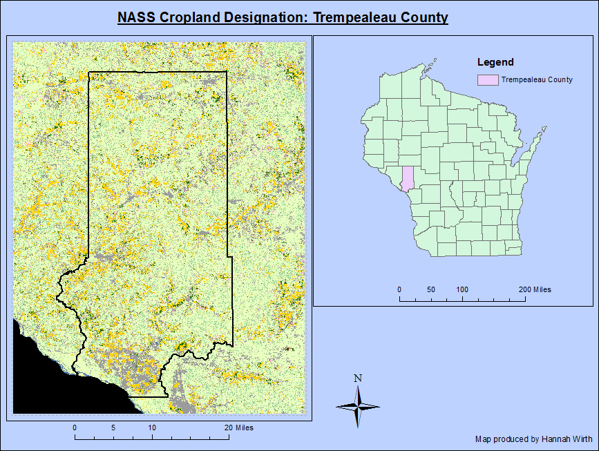
Figure 1: Cropland Data for Trempealeau County

Figure 2: Land Cover Data for Trempealeau County

Figure 3: Digital Elevation Model (DEM) for Trempealeau County

Data Accuracy:

By looking at the metadata for the data downloaded, it shows information about the actual data gathered. It also shows how accurate and reliable the data is. This is helpful to know about any limitations or coordinate system projections for the future. Below is a list of the data gathered. For each data set, we had to find the scale, effective resolution, minimum mapping unit, planimetric coordinate accuracy, lineage, temporal accuracy and attribute accuracy. If there was no information for a category, it is denoted with N/A.

Conclusion: The ability to download free data off of the website from credible sources is a great skill to have. Most of the data that will be needed to complete this project has now been downloaded. It is all stored in a geodatabase specifically for this project. Although the downloading of data can be frustrating, it is good practice. I am very interest and curious to see what the final results show about the suitability of frack sand mining in Trempealeau County.

Websites:

USDOT:  http://www.rita.dot.gov/bts/sites/rita.dot.gov.bts/files/publications/national_transportation_atlas_database/index.html
USGS: http://nationalmap.gov/about.html
USDA: http://datagateway.nrcs.usda.gov/
USDA NRCS Soil Survery: http://websoilsurvey.sc.egov.usda.gov/App/HomePage.htm
Trempealeau County Geodatabase: http://www.tremplocounty.com/tchome/landrecords/

Python Script

Python Script #1

The goal for exercise 5 part three was to write a new Python script to project, clip, and load all the data into a geodatabase. 

Python is a general-purposed programming language. It is designed to have readable code and syntax that programmers can use. In our GIS II class, we used Python to  write scripts for our geodatabases in ArcGIS. For this specific assignment, we had to download multiple data and rasters to analyze Trempealeau county. We used Python for projecting the rasters into the Trempealeau geodatabase. 

Figure 1: This is a screenshot of the completed Python script 

Above is the completed Python script. The Python troubleshooting took quite a long time and tested my patience. When there were no longer any errors with the script, it was complete.

Python Script #2

The goal of exercise 7 was to write a python script to prepare the data for network analysis. Python Scripter was used to write the script. The script consisted of selecting the mines, multiple queries, and selecting by location. I used select by location to find the mines that were active, within 1.5 km of a rail system, and a mine that does not have a rail loading station on-site.

Figure 2: This is the completed Python script for exercise 7

Writing the script was frustrating, but once I got the hang of it, it was easier to write. The script was broken down into    main parts. Step one was to set up the environments and prepare for writing the SQL statements. Step two was to write three SQL statements. Step three was to create new feature from the SQL expressions. Step four was to select by location to find the number of mines that are active, within 1.5 km of a rail system, and find mines that do not have a rail loading station on-site. I found 35 mine systems that require trucking to and from their sites. 

Python Script #3

This is the last and final Python script for GIS II. I went through the same workflow as I did in ArcMap. This script created a new raster overlay based on the same criteria, but one weighted 1.5 times more than the others. I chose to weight distance from streams higher. The Python script is shown below.

Figure 3: This is the completed Python script for exercise 8